[ML] 타이타닉 생존 예측 분류모델

간단한 분류모델인 titanic 데이터를 활용한 생존 예측 분류 모델에 대하여  머신러닝 프로세스를

알아보도록 하겠습니다. 

매트릭의 성능지표 개선보다는 머신러닝 프로세스, 모델 훈련, 모델 비교 하는 방법에 대해서 알수 있습니다.

다양한 머신러닝 모델에 대해서 반복적으로 경험하다 보면 프로세스가 익숙해 질것이니 코드를 수행해

보시면서 익숙해 지시기 바랍니다.

 

1. 라이브러리 import

import pandas as pd # 판단스
import seaborn as sns #그래프
from sklearn.model_selection import train_test_split #훈련 및 테스트 분류
from sklearn.preprocessing import LabelEncoder # 범주형 인코딩
from sklearn.metrics import accuracy_score # metric
from sklearn.linear_model import LogisticRegression #모델 
from sklearn.ensemble import RandomForestClassifier, GradientBoostingClassifier #모델
from xgboost import XGBClassifier #모델
from lightgbm import LGBMClassifier #모델

 

2. 데이터로드 및 출력

df = sns.load_dataset('titanic')
df.head()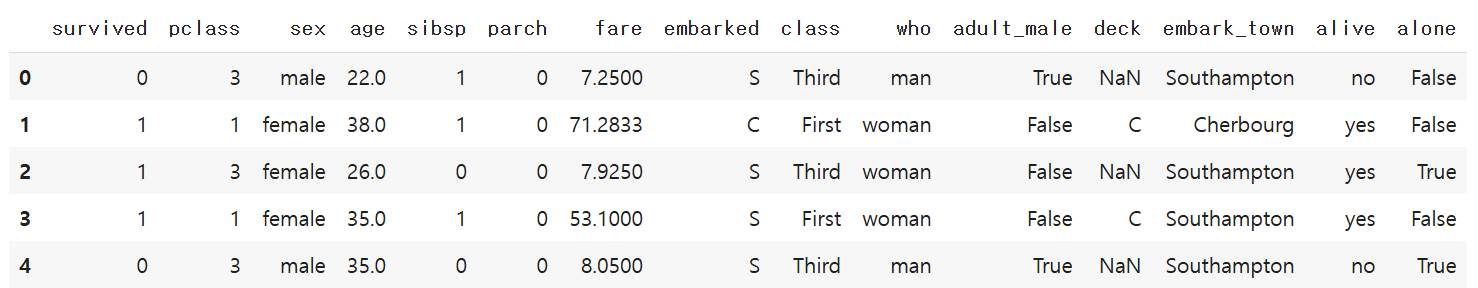

 

3. 데이터 통계량

dfSummary(df)로 다양한 통계 데이터를 볼수도 있습니다.

df = df[['survived', 'pclass', 'sex', 'age', 'sibsp', 'parch', 'fare', 'embarked']]
df.describe(include='all').T  # 범주형 데이터도 같이 보여줌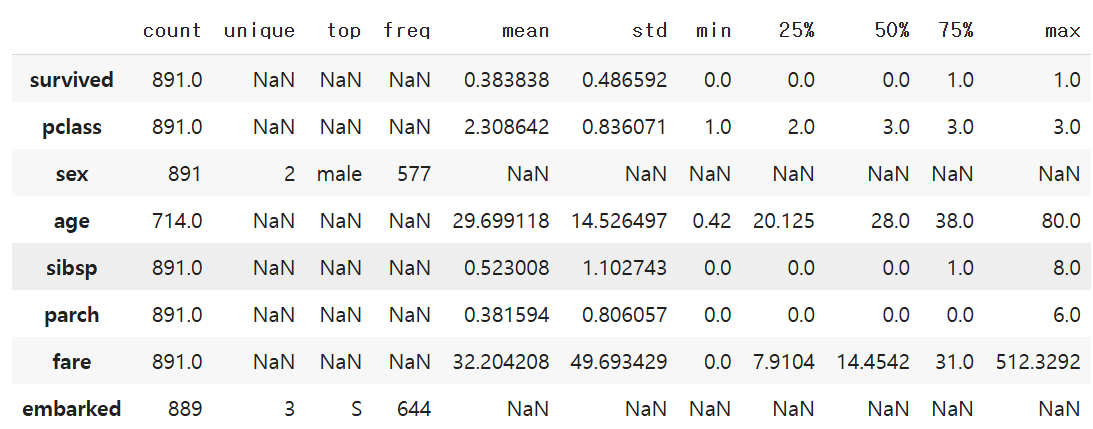

count에 일부 컬럼은 null임으로 알수 있습니다.

평균,중앙값,최빈도,보간법 등 다양한 방법으로 치환할 수 있습니다.

(이번에는 삭제하는 방법으로 간단히 처리하겠습니다.)

 

4. 데이터 전처리

df = df.dropna()

# 범주형 변수 인코딩
label_encoders = {}
for col in ['sex', 'embarked']:
    le = LabelEncoder()
    df[col] = le.fit_transform(df[col])
    label_encoders[col] = le

# 특성과 타겟 분리
X = df.drop('survived', axis=1)
y = df['survived']

# 학습/테스트 데이터 분할
X_train, X_test, y_train, y_test = train_test_split(X, y, test_size=0.2, random_state=42)

일반적으로 모델은 범주형 변수를 수치형 변수로 변경을 하여야 합니다.

이때  Label Encoder, One Hot Encoding, Ordinal Encoding가 있습니다.

인코딩에 대해서도 향후 별도로 정리하도록 하겠습니다.

 

 

  5. 모델 학습

# 모델 정의
models = {
    "Logistic Regression": LogisticRegression(max_iter=1000),
    "Random Forest": RandomForestClassifier(n_estimators=100, random_state=42),
    "Gradient Boosting": GradientBoostingClassifier(random_state=42),
    "XGBoost": XGBClassifier( eval_metric='logloss', random_state=42),
    "LightGBM":LGBMClassifier(
                random_state=42,
                min_child_samples=5,    # 작은 leaf에도 분할 허용
                min_split_gain=0.0,     # 정보 이득이 낮아도 분할 허용
                verbosity=-1            # 경고 메시지 출력 안함
                  )
}

# 모델 학습 및 평가
results = []
for name, model in models.items():
    model.fit(X_train, y_train)
    y_pred = model.predict(X_test)
    acc = accuracy_score(y_test, y_pred)
    results.append((name, acc))

모델 5개을 훈련하고 평가지표로 정확도(accuracy)를 계산함

 

6. 결과 출력 및 시각

import matplotlib.pyplot as plt
plt.rc('font', family='NanumBarunGothic') # 한글
# 결과 정렬 및 출력
results.sort(key=lambda x: x[1], reverse=True)

print("모델 정확도 비교 결과:")
for name, acc in results:
    print(f"{name}: {acc:.4f}")

# 가장 높은 정확도를 가진 모델
best_model_name, best_acc = results[0]
print(f"\n가장 높은 정확도 모델: {best_model_name} (정확도: {best_acc:.4f})")

# 결과를 DataFrame으로 변환
results_df = pd.DataFrame(results, columns=["Model", "Accuracy"])
# 정확도 기준으로 정렬
results_df = results_df.sort_values(by="Accuracy", ascending=True)
# 시각화
plt.figure(figsize=(10, 6))
bars = plt.barh(results_df["Model"], results_df["Accuracy"], color='skyblue')
# 정확도 수치 추가
for bar in bars:
    width = bar.get_width()
    plt.text(width + 0.005, bar.get_y() + bar.get_height()/2, f"{width:.4f}", va='center')
plt.xlabel("Accuracy")
plt.title(" 모델별 타이타닉 생존 예측 정확도 비교")
plt.xlim(0, 1)
plt.tight_layout()
plt.show()

모델 정확도 비교 결과:

Logistic Regression: 0.7972

Random Forest: 0.7902

LightGBM: 0.7902

Gradient Boosting: 0.7692

XGBoost: 0.7413

가장 높은 정확도 모델: Logistic Regression (정확도: 0.7972)

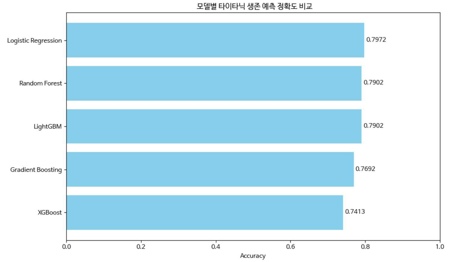
간단히 데이터 전처리 없이도 80%가까이 정확도를 나타내고 있습니다.

실제 random forest는 범주형 데이터를 그대로 사용해도 됩니다.(label encoder 불필요)